Sensory dominance in extended haptics: Applied stochastic method
Article information
Abstract
This study measured haptic extra accuracy, that is, judging one hit position in a hand-held object. Primarily, which factors are associated with the estimation of the contact position when an impact is made on the grasped implement. Data were collected from 20 participants and their extended haptic accuracy were analyzed using a discrete numerical state, as well as the stochastic evolutionary possibility. Analyzations proved that perceived accuracy influenced not only the stimulus magnitudes distinguished by the coefficient of restitution, but also the distributions of the encoded impressions by the rotational inertia. In particular, stochastic analysis confirmed that perceiving the location of the effect of grasped objects is more constrained by kinesthetic oriented property than by the cutaneous oriented gain in arbitrarily conflicted circumstances. The results from the analyzations suggest a broader hypothesis for further research into the effects of inertia tensor related to haptic spatial accuracy in a hand-held object.
Introduction
In psychology, biology, engineering, and even work on robots, integration through touch is critical to discovering the world (Bicchi, Gabiccini, & Santello, 2011). The sense of touch is considered a trademark of a process that can inform and guide growing interest in the search for rational principles. With regard to what information can be derived and how that information can be best obtained, the sense of touch offers a means to understand both crucial and elemental sensory mechanisms.
To date, various studies have demonstrated that the physical properties of an object represent crucial aspect of perceived touch sensations (Amazeen & Turvey, 1996; Charpentier, 1981; Weber, 1834/1978). The basis of this mechanical ability of this characteristic (inertia tensor) is considered an invariant of extra perception dynamics (Solomon & Turvey, 1988; Burton, Turvey, & Solomon, 1990). It is however well documented that haptic perception may not merely be mechanical contact based on the tensile states of muscles, tendons, and fascia, but rather patterns the ensemble activity of receptors (Fonseca & Turvey, 2006). For example, perceived heaviness of a hefted object did not correspond simply to the object’s length, orientation, and weight (Weber, 1834/1978). More over, when different senses (i.e., modalities) are conflicted, the impression of one of the senses is uniquely constrained by the other (i.e., Size-Weight Illusion; Ellis & Lederman, 1993).
Inspired by the developments to naturally generalize such biases so that they uniformly maximize mechanical production (Turvey, 1996), a significant issue in touch science involves understanding how people localize discrete contact points in a space external to the body; i.e., “Where was I touched?” For daily processes, other types of haptic perception, such as determining where in the space external to the body a stimulus is being experienced, can be expected. Researchers on haptic space perception have produced some interesting phenomena related to the question “What is the frame of reference within which localization occurs?” They proposed that determining the contact site and localizing within an external space are grounded in the contact between the skin and an external object, but the frames of reference might not be different (Lederman & Klatzky, 2009).
According to insights offered by Weber (1834/1978) related to perceived heaviness, sensing perceived heaviness during dynamic touch is done using the pressure exerted on the skin. As pressure is directly related to the mass of the object causing it, perceived heaviness was a function of the cutaneous sense of pressure as determined by the mechanoreceptor’s vibration sensing ability of the skin (Welfe et al., 2008). Likewise, the ordinary perception abilities of many species (i.e., spiders and scorpions), are induced on the basis of vibrations on the surfaces on which they stand and move (Barrows, 1915; Witt, 1975). Stevens & Rubin (1970) also emphasized that when the mass of an object was constant, the decreasing density caused by an increasing in the object’s volume led to less pressure being exerted on the skin. This evoked a perception of less heaviness by participants.
The large capacity of humans to capitalize on dynamics arising from contact with objects and nearby surfaces suggests that others froms (i.e. wave) may serve as a mechanical kernel in an exploitabel medium to perceive objects (Kinsella-Shaw & Turvey, 1992). Although research related to haptic perception has hinted at a possible deep connection between kinesthetic properties and cutaneous gains (Park & Kim, 2014; Stevens & Rubin, 1970; Weber, 1834/1978), valid scores of a function have mainly been estimated by measuring only one aspect between the two modalities. The comprehensive formal relationship and dominance between these inputs has not been addressed (Millar, 1976; Zhu, Shockley, Riley, Tolston, & Bingham, 2013), though perceiving spatial surface layout was reported under conditions considering the distance from the hand and the magnitudes of the gaps between surfaces (Barac-Cikoja & Turvey, 1991; Carello, Fizxpatrick, & Turvey, 1992).
The goal of this study is therefore to identify such a relationship through a generalization of mechanical properties previously found by the authors (rotational inertia) to cause the “Where was I touched?” haptic circumstance. In addition, the present study aims to determine which element in a conflicted situation plays the main role. To assesee which factors are associated with the assumptions, relative probability and evolution of the probability were used, which is considered as an ideal tool for estimating (or likeliness) continous (or discrete) variables, to determine the response required based on the following questions. (i) Can extra perception dynamics (judging a hit position of a rod) be affected by the stimulus magnitude? (ii) Can extra perception dynamics be affected by the stimulus distribution? (iii) Can extra perception dynamics be derived from the mechanical properties of the distribution rather than simply the magnitude of the stimulus, as the most critical characteristics related to hand-held object perception (heaviness) has been affected by the rotaoinal inertia (not simply weight of the object)?
Within this line of reasoning, the following hypotheses could be drawn. First, the mechanical property of (a) the amount of stimulus (conditioned by coefficient of restitution) will be significant for when judging a contact position of a rod. Second, (b) the amount of distribution (conditioned by rotational inertia) will be significant when judging a contact position of a rod. Third, (c) there will be dominant effect for accuracy in an arbitrarily conflicted circumstance between the two modalities (kinesthetic oriented rotational inertia vs. cutaneous oriented coefficient of restitution).
The expectation should be that if these mechanical factors are investigated and the different levels are captured, the significance could be suggested as a broader hypothesis for further research. These extended perception-associated features stemming from the different components can contribute to the effects of the haptic accuracy in the hand-held object. The results will lead to various estimates of system functions providing an account of generalization that accommodates a variety of aspects.
Methods
Participants
The data used in this experiment were collected from undergraduate students (N=20, 10 female, 10 male). The mean age was 20.5 years old (range 18 – 23). Participants at the University of Connecticut (Storrs, USA) were enrolled in an introductory course and received credit for their participation. All participants had normal mobility of their right arms, and individuals were excluded through self-reported acute or chronic physical and psychiatric disorders [three participants were eliminated by the criteria of dominant hands (two = left handed) and a self reported disorder (one = sprained ankle)]. All participants provided written informed consent, and the study was approved by the relevent local ethics committee (SNUIRB No.1509/002-002) and conformed to the ethical standards of the 1964 Declaration of Helsinki (Collaborative Institutional Training Initiative Program, report ID 20481572).
Apparatus and procedure
The task set in the experiment was the same in every case: Determining the strike position of a rod with a ball and reporting the distance on the rod using a black arrow attached to a strand line (at the opposite hand) at the point of contact. A participant was seated in a chair with the right forearm supported out to the elbow. During each trial, a custom-made wooden frame (object: 40 cm rod, 1 cm diameter, 180 g) was placed on the right-hand side of a participant. Participants wore headphones to block potentially distracting background noise and contact sounds from the set, and were asked to hold the rod on the side obscured by an opaque curtain to block visual stimuli.
They were instructed to grasp the rod comfortably in a fixed manner as directed by an assistance, with the thumb and index finger securely closing toward the oriented rod direction to minimalize the ability of the hand to close on an object corresponding to a normalized range from 0 to 1 (see Appendix 1 for more detail). A monitor in front of the participant displayed a corresponding image so that they were aware of the spacial area of the rod and indicated the contact point using a driving pulley (at the opposite hand) which was attached to a black arrow on a strand line (see Appendix 2 for the experimental setup).
In each instance, the experimenter initiated the trial once a participant was ready. An assistant released a object (i.e., a ball) from a certain height (10, 20, and 30 cm) to fall a particular distance (10, 20, and 30 cm) onto the rod (see Appendix 3 for more detail). The contact between the fallen obejct and rod occurred three times in a completely randomized order for each participant at each distance and at each height (27 trials = 3*3*3). The participants were given five practice trials, on completion of each test. The object distances and falling height of the ball in the practice session however, differed from those of the actual experiment. The participant was encouraged to take enough time to get haptic feedback from the hand in which the object was grasped and report using their non-dominated arm to position the side arrow. The initial position of the arrow used for reporting was randomized across trials for each participant. The assistance (calculating system) of the object determined the difference in distance between the actual contact site and the reporting arrow site. The difference obtained was quantified with a grid pattern map which was marked on both the object and the strand line linked to researcher’s computer. The size (mm) of the absolute error (AE= Σ│Xi – T│ / n) between an actual hit position and the perceived/designated position was transmitted by using a custom made linking system that was previously devised. The size of magnitude and contact point with the rod applied point on the rod were also transmitted by the linking system and calculated as unit per SI.
No further instructions or feedbacks as to the accuracy, amplitude, or frequency of results during the trials were communicated to the participants. Each experimental session lasted approximately 30 minutes. After the final trial, each participant was shown how well he or she had performed on the experiments through the researcher’s computer.
Analysis
Relative probability densities: Mean value and variance are measures of central tendency and variability for continuous (discrete) variables defined on the real line. They may also be applied to variables under certain circumstances. In general, statistics should be applied to variables to determine the center and the variability of probability densities and samples. Among several available measures, this analysis focuses mainly on the deterministic system, which state is described by a discrete numerical state variable. This method explains whether there is a consistent difference between the data. If so, a scientific guess can be made as to which data set belongs to what significant effect in experimental conditions.
First, each accuracy was defined as the absolute error between an actual contact position and the perceived designated position, after which these sizes were converted to a discrete state unit (1=distance within 0~1 cm, 2=distance from 1 cm ~ 2 cm). This allows us to see each variables’ proportion (percentage) of occurrences of that outcome in the statistical ensemble as follows;
Where hj is the number of occurrences of a repeating event–usually called frequency during the period of time. In statistics, this occurrence of an event (j) is the number (k) of times the event took place in an experiment.
Where relative frequency (fj) is reflected by how often something happens divided by all outcomes. This event refers to the absolute frequency (hj) normalized by the total number of events (N). The relative frequency, also known as empirical (experimental) probability is represented as follows;
Where Pj is the ratio of the number of outcomes (
Next, to estimate how many realizations per measurement unit occur on a continuous level, a probability function based on the construction of a density for these data sets can be used as follows;
Evolution of the probability: We are always faced with uncertainty, ambiguity, and variability. Although we now have unprecedented access to information, being able to accurately predict the future is still almost impossible. The Monte Carlo simulation (based on the Markov chain model) allows us to see all possible outcomes and assess the possible impacts of the outcomes that may occur in the future, using not only information from the current state, but also from the sequence of events that preceded it. To address this likelihood, the haptic accuracy state variable was continuously placed as a probability density and variability according to the discrete time series. The relative ratio of the differences between all the designated conditions and the ratio of each condition were calculated using the Markov chain model based joint probability as follows;
Where P is the probability that the system is in the state (k) at the time step (n) and in the state (j) at a next time step. The assumption for probability could not express how to create probabilities for combined events such as P[A ∩ B] or for the likelihood of an event A, given that it is known that event B occurs. For instance, let A be the state of distribution effect accuracy (within SD±1) at one condition and B be the state of non-distribution effect accuracy for the other condition. Does knowledge of haptic accuracy at the one condition change the belief that it will still be accurate for the other condition? That is, P[B] , is the probability that the accuracy of the other condition is ignoring information on whether it is accurate at the condition. This differs from, the probability that it is accurate at the other condition given that it is accurate at the time step (called conditional probability of B given A). It is quite likely that P[B] and P[B | A] are different.
This probability density and the probabilities of the two variables can be calculated by generating the data (X1) and (X2) for a participant. Using this information, the time-evolution of a system can be modeled to occupy each of a countable number of states (discrete set of states) about a continuous time step, where switching between states is treated probabilistically. In this case, the master that describes the evolution of the probability p(j, t), where t is time, is defined by
Here, w(j←k) denotes the transition rate from k to j. This modeling will allow the progression of haptic accuracy dependency (progression of performance probability) as an application. Intuitively, what can we say about this evolutionary probability
Results
Relative probability
Many inputs evoke a complicated system of orienting reflexes in an organism. These orienting reactions are of course subject to their intensity, and roughly corresponds to that of the inputs. This gradually changes when these actions have been repeated frequently. It is probably that, the higher the relative frequency of an event, the more certain we are that the event will occur. To estimate this measurement, a probability function based on the construction of density for these data sets was calculated.
The results show the deviation of the performance parameter for the interaction between error and variance of the error from the different heights [F(2, 71) = 26.951, = η2 13.475 (p < 0.001), (Pearson Correlation R = - .61)]. In addition, these results also reflect the deviation of the performance parameter for the interaction between error and variance of the error from the different distances [F(2, 71) = 28,865, = η2 14.433 (p < 0.001), (Pearson Correlation R = - .63)] (see Appendix 4 for the statistical approaches). The analyses show that observers influenced not only the stimulus magnitudes distinguished by the coefficient of restitution, but also the distributions of the encoded impressions by the distance from the hand to the impact (see Table 1).

Comparative estimation of the parameter between heights and distances
For more detail, these results were further investigated to deal with matters such as the conflicted circumstances between the two modalities. Specifically, the participants’ judgment of the contact point can also be derived from the mechanical properties of the distribution rather than the the magnitude of the stimulus. Table 2 shows which parameter plays a more significant role in the arbitrarily estimated comparisons between the two different combinations. Both densities (error size estimation, error variance estimation) illustrate that the combination of the height 10 cm and the distance 30 cm caused better accuracy with less variance, than the combination of the height 30 cm and the distance 10 cm. The mechanical foundation of the stimulus distribution (conditioned by the rotational inertia as more kinesthetic oriented gain = relatively many scores at the extreme ends) makes its influence more significant than its impulse magnitude (conditioned by coefficient of restitution as more cutaneous oriented gain = relatively few scores at the extreme ends) for accuracy in arbitrarily conflicted circumstances between the two modalities. Likewise, the most critical characteristic in the hand-held object’s perceived size-weight ratio was not the object’s weight, but rather the rotational inertia in the conflicted circumstance (Charpentier, 1981). Localized discrete contact points in the grasped implement can also be derived from the same mechanical property of the distribution rather than from the magnitude of the stimulus.

Calculating conditional probability between H1+D3 and H3+D1
Evolution of the probability
In the discrete time series of a Markov process based on the model, the probability of a particular state in the future behavior depends only on the current state and not on the past. Since we can iterate a Markov process from an initial state numerically, we might be observing an estimation of parameters. By repeating the steps in previous procedures and making panels for P (distribution, not distribution), we can state whether we get the impression that the graphs do not change much when we look at different sample sizes. If this does not change much, then we can say that we have good approximations for the N to infinity limiting case. These estimates are maximum likelihood estimators (MLEs) for those parameters where the likelihood of observing a given data set is maximal.
Table 3 shows that especially the error variance becomes more significant based on conditional probability, F(1, 15) = 17,030, = η2 .549 (p < 0.001). As it is, the time-evolution of a system was analyzed to occupy each one of a countable number of states (discrete set of states) about a continuous time step, and where switching between states is treated probabilistically.

Comparative estimation of the parameters between heights and distances. P(xj)=Probability Markov Chain model
This additional analysis shows that the answer to the hypothesys (c) which the dominant state between conditions can be estimated from a different viewpoint so that it is more clear which influence would be more robust. The results, in conjunction with a prior analysis on the relative probability, suggest that the standard property (rotational inertia) of the hand-held object can be detected as the crucial feature in this perceived position accuracy as well (see the Table 3). Notably, both mechanical source of information could be perceptually independent and combine additively, although it could be the case that one source or the other dominates (see the Table 4, and Figure 1).

Calculation for transition probability. E_S=error size parameter based. E_V=error variance parameter based. Model that exhibits only three steps of transitions, where t is time and j is the discrete state defined by (1=10 cm, 2=20 cm, 3=30 cm). H=conditional height for the coefficient restitution, D=conditional distance for the pressure distribution. The left table denotes modeling for progression on the basis of conditional probability {Ω [P(x1,x2)] = 1, 2, 3}
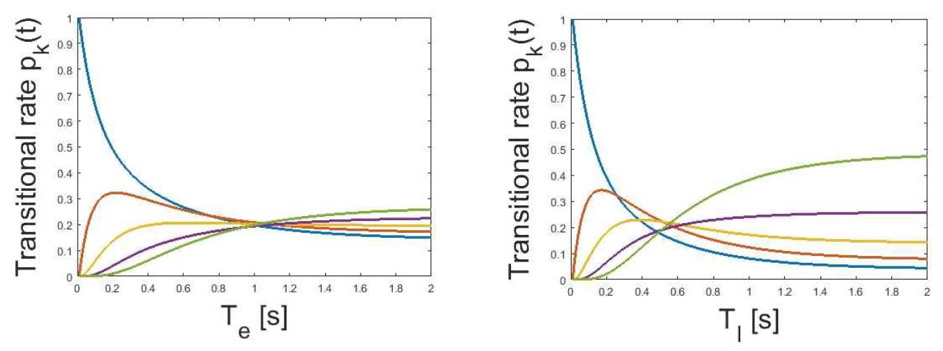
The transitional rate (probability) of the continuous time process. The plot of the left side represents the transitional rates of states with height e : d d t p j , t = . 008 I : d d t p j , t = . 03
Discussion
The goal of this study was to conceptually link the role of the familiar classical concept of rotational inertia in a “Where was I touched?” circumstance. This approach was inspired by the suggestion that dynamic aspects of touch, such as the relative mass of colliding objects (Todd & Warren, 1982) or the mass of lifted objects (Bingham, 1987), can be determined despite the fact that the other modality is conflicting with the encouraging viewpoint.
The results of this observation, that is, (a) perceiving the location of the impact of grasped objects, were virtually identical in respect of its response to a given applied impulse. When an object experiences more coefficient of restitution in response to a given impulse, there is an expectation that it will also be perceived as stronger. Likewise, (b) the observation was compatible when faced with a different location of the contact since observers expect a closer location of the contact point to be weaker than one that is further away. Another interesting observation was that (c) the influence from the stimulus magnitude seems to be weaker than the location of the stimulus when presented with the concurrent manipulation of both modalities. That is, stimulus distribution (from the location) has a stronger influence if the analysis specifies an object that rotates (or vibrates) differently in response to the same applied impulse of a grasped object.
Physical property (Inertia tensor): Here, one of the basic properties can explicitly propose a progressed step in the form of simple physical systems as indicated below. Apparent perception can be described as a function of the variable and constant parameter (ψ = Kϕβ). Where ψ is apparent perception, ϕ is the variable, β is the slope, and K is a proportionally constant parameter. However, the perception can be determined by a function of the constant (not variable) if given the same variables (ψ = b – a logV) (Stevens & Rubin, 1970). Where ψ is the perceived impression (i.e., heaviness). V is the constant, a is the coefficient slope, and b is the additive constant.
Specifically, the perceived impression of a hefted object did not correspond simply to the object’s mass (or variable), but instead to changes in the constant –location of the object’s center of mass that accompanied changes in the location of the rotation point (ψ ≈ M × (CM – O)2) (Amazeen & Turvey, 1996). Where ψ is perceived heaviness, M is the mass of the object, CM is the location of the object’s center of mass, and O is the location of the rotation point. Under this assumption, the perceived impression is uniquely constrained by the eigenvalues of the inertia tensor (Amazeen & Turvey, 1996; Carellro, Thuot, Anderson & Turvey, 1999; Stroop, Turvey, Fitzpatrick & Carello, 2000; Streit, Shockley & Riley, 2007; Shockley Morris & Riley, 2007; Harrison, Hajnal, Goodman, Isenhower & Show, 2011).
Under this assumption, the result of this study may be expanded by the property of the apparent perception when it comes to uniquely constrained by the physical property of the eigenvalues (location of the object’s center of mass from the site of the rotation point) into the perceived position aspects. In other words, the perceived position accuracy of the hand-held object did not correspond simply to the amount of the parameter variable (coefficient of restitution), but instead corresponded to changes in the location of the contact point that accompanied changes in the location of the center of pressure [Ap = Ce × (CP –O)2]. Where Ap is the perceived spatial accuracy, Ce is coefficient restitution of the object, CP is the location of the center of pressure, and O is the location of the rotation (grasp) point.
By generalization, the haptic perception of extended spatial accuracy may correspond to equal differences among the logarithms of the constants (K = CP) or, in other words, a logarithmic function uniquely constrained by the eigenvalues of the inertia tensor [Ap ≒ I, I = mass × (CM –O)2]. We now know that Ap ≒ I. This, in fact, is the formal definition of the property used by the S-W illusion investigation (Davis & Brickett1977; Charpentier, 1981), what is called a precise control over the grasped non-visible objects (Amazeen & Turvey, 1996). The present study found that the property takes on a particular patterning in a comprehensive extended spatial haptic. The conjecture is that for a given applied pressure at the same impulse magnitude (=Ce) as the parameter variable, haptic spatial accuracy (=Ap) will increase as the rotational inertia (=I) increase.
Apparently, a detected physical property must influence the perception of where in the space external to the body a stimulus from a wielded object is being received in a manner consistent with the inertial model. Inspired by Stevens & Rubin’s (1970) idea and reinforced by Weber’s (1834/1978) deep connection between kinesthetic properties and cutaneous gain (if the object lies on a larger skin surface rather than a smaller one, the sensation is similar though not quite equal), this result of the perceived impressions of a hefted object seems to correspond to their frames of reference. This might not be different from changes in the location of the object’s center of mass that accompanied changes in the location of the rotation point (Anderson, 1970).
Psychological Property (estimating two conflicted inputs): The point of view that the study established here holds some possibility of a better understanding of the haptic system. The assumption is that haptic accuracy traces are associated not only with physical traces, but also with the system of psychological accuracy coordinates. By this, the present study does not mean that the accuracy has one particular subsystem in haptic perception. On the contrary, these experiments conclusively show that this is not the case. Rather, when the haptic accuracy trace is formed, it is integrated with invariant characteristics of the physical property called rotational inertia, which gives it position in relation to the other (pressure distribution) associated psychological traces (Kinsella-Shaw & Turvey, 1992).
When a person faces an object while exploring it with their modalities, they receive information for estimating the properties of the object. The estimate of a surrounded property by a sensory system can be represented by [
The results of the present study suggest that this system is a combination of subsystems so linked together that the inputs furnished by the actual performance of certain perceptions are required to bring about other perception. What then determines the order? Essentially, such positions offer no solution to the problem of temporal integration. The thought is neither muscular contraction nor image, but can only be inferred as a determining tendency. The study further asserts that the set does not have a temporal order–in other words, that all of its elements are co-temporal. The form of expression of an idea can be changed depending on the case with which different accuracy rules may be utilized to express evidence that the temporal integration is not inherent in the preliminary organization of the idea. The haptic arrangement of these results is obviously not due to any direct associations of the input itself with other inputs, but rather to meanings that are determined by some combined relations. The system can take its position only when a particular meaning becomes dominant. This dominance is not inherent in the modalities themselves.
Conclusions and practical applications
Our sensory system must be regarded as a great network of reverberatory circuits that are constantly active. A new stimulus does not excite an isolated reflex path, rather, most produce widespread changes in the pattern of excitation throughout a whole system of already interacting stimuli. Even identical cells in a particular region of the brain cortex participate in a great variety of activities (Lashley, 1951). A common theory about classical exploration of thought and discussion, concerns the danger of complacency—in the absence of challenge, one’s opinions, even when they are correct, grow weak and flabby. Even under the best circumstances, one’s opinion tends to embrace only a portion of the truth, and because opposing opinions rarely turn out to be completely erroneous, it is crucial to supplement one’s own opinions with an alternative point of view.
In spite of its present inadequacy, a haptic study has been improved by the belief that they are linked in a relatively isolated conditioned response and that they are activated when the particular reactions (with which they are directly associated) are called out. Such a view is incompatible with the widespread effects of stimulation, which can be demonstrated by recent evidence from neurological and psychological recording of the haptic system. To rule out the above-mentioned assumption of this study, the suggested expectation would require additional manipulation of the conflicted virtual setting within the present paradigm. Such an implementation would allow more influence of the invariant physical property to be demonstrated from impacts of psychological phenomena.
Acknowledgements
This research was supported under the framework of International Cooperation Program managed by National Research Foundation of Korea (Grant Number: 2016K2A9A1A02952017).
References
Anderson, N. H. (1970). Averaging model applied to the size-weight illusion. Perception & Psychophysics, 8(1), 1-4.
10.3758/BF03208919.Amazeen, E. L., & Turvey, M. T. (1996). Weight perception and the haptic size–weight illusion are functions of the inertia tensor. Journal of Experimental Psychology: Human perception and performance, 22(1), 213.
10.1037/0096-1523.22.1.213.Bajcsy, R. (1988). Active perception. Proceedings of the IEEE, 76(8), 966-1005.
10.1109/5.5968.Bicchi, A., Gabiccini, M., & Santello, M. (2011). Modelling natural and artificial hands with synergies. Phil. Trans. R. Soc. B, 366(1581), 3153-3161.
10.1098/rstb.2011.0152.Barac-Cikoja, D., & Turvey, M. T. (1991). Perceiving aperture size by striking. Journal of Experimental Psychology: Human Perception and Performance, 17(2), 330.
10.1037/0096-1523.17.2.330.Barrows, W. M. (1915). The reactions of an orb-weaving spider, Epeira sclopetaria Clerck, to rhythmic vibrations of its web. Biological Bulletin, 29(5), 316-332.
10.2307/1536407.Burton, G., Turvey, M. T., & Solomon, H. Y. (1990). Can shape be perceived by dynamic touch?. Attention, Perception, & Psychophysics, 48(5), 477-487.
10.3758/BF03211592.Bingham, G. P. (1987). Kinematic form and scaling: further investigations on the visual perception of lifted weight. Journal of Experimental Psychology: Human Perception and Performance, 13(2), 155.
10.1037/0096-1523.13.2.155.Carello, C., Fitzpatrick, P., & Turvey, M. T. (1992). Haptic probing: Perceiving the length of a probe and the distance of a surface probed. Attention, Perception, & Psychophysics, 51(6), 580-598.
10.3758/BF03211655.Carello, C., Thuot, S., Anderson, K. L., & Turvey, M. T. (1999). Perceiving the sweet spot. Perception, 28(3), 307-320.
10.1068/p2716.Charpentier, A. (1891). Analyse experimentale de quelques elements de la sensation de poids. [Experimental analysis of some elements of weight sensations] Archives de Physiologie Normales et Pathologiques. 3, 122–135.
Davis, C. M., & Brickett, P. (1977). The role of preparatory muscular tension in the size-weight illusion. Perception & Psychophysics, 22(3), 262-264.
10.3758/BF03199688.Ellis, R. R., & Lederman, S. J. (1993). The role of haptic versus visual volume cues in the size-weight illusion. Perception & psychophysics, 53(3), 315-324.
10.3758/BF03205186.Ernst, M. O., & Banks, M. S. (2002). Humans integrate visual and haptic information in a statistically optimal fashion. Nature, 415(6870), 429-433.
10.1038/415429a.Fonseca, S., & Turvey, M. T. (2006). Biotensegrity perceptual hypothesis: A medium of haptic perception. In North America Meeting of the International Society for Ecological Psychology. Cincinnati, Ohio.
Gibson, J. J. (1962). Observations on active touch. Psychological review, 69(6), 477.
10.1037/h0046962.Harrison, S. J., Hajnal, A., Lopresti-Goodman, S., Isenhower, R. W., & Kinsella-Shaw, J. M. (2011). Perceiving action-relevant properties of tools through dynamic touch: Effects of mass distribution, exploration style, and intention. Journal of Experimental Psychology: Human Perception and Performance, 37(1), 193.
10.1037/a0020407.Kinsella-Shaw, J. M., & Turvey, M. T. (1992). Haptic perception of object distance in a single-strand vibratory web. Perception & psychophysics, 52(6), 625-638.
10.3758/BF03211700.Lashley, K. S. (1951). The problem of serial order in behavior. In Cerebral mechanisms in behavior (pp. 112-136).
Lederman, S. J., & Klatzky, R. L. (2009). Haptic perception: A tutorial. Attention, Perception, & Psychophysics, 71(7), 1439-1459.
10.3758/APP.71.7.1439.Millar, S. (1976). Spatial representation by blind and sighted children. Journal of Experimental Child Psychology, 21(3), 460-479.
10.1016/0022-0965(76)90074-6.Nelson, M. E., & MacIver, M. A. (2006). Sensory acquisition in active sensing systems. Journal of Comparative Physiology A, 192(6), 573-586.
10.1007/s00359-006-0099-4.Park, C., & Kim, S. (2014). Haptic perception accuracy depending on self-produced movement. Journal of sports sciences, 32(10), 974-985.
10.1080/02640414.2013.873138.Sanso, R. M., & Thalmann, D. (1994, August). A hand control and automatic grasping system for synthetic actors. In Computer Graphics Forum (Vol. 13, No. 3, pp. 167-177). Blackwell Science Ltd.
10.1111/1467-8659.1330167.Solomon, H. Y., & Turvey, M. T. (1988). Haptically perceiving the distances reachable with hand-held objects. Journal of experimental psychology: Human perception and performance, 14(3), 404.
10.1037/0096-1523.14.3.404.Stevens, J. C., & Rubin, L. L. (1970). Psychophysical scales of apparent heaviness and the size-weight illusion. Perception & Psychophysics, 8(4), 225-230.
10.3758/BF03210210.Streit, M., Shockley, K., & Riley, M. A. (2007). Rotational inertia and multimodal heaviness perception. Psychonomic bulletin & review, 14(5), 1001-1006.
10.3758/BF03194135.Streit, M., Shockley, K., Riley, M. A., & Morris, A. W. (2007). Rotational kinematics influence multimodal perception of heaviness. Psychonomic bulletin & review, 14(2), 363-367.
10.3758/BF03194078.Stroop, M., Turvey, M. T., Fitzpatrick, P., & Carello, C. (2000). Inertia tensor and weight-percept models of length perception by static holding. Journal of Experimental Psychology: Human Perception and Performance, 26(3), 1133.
10.1037/0096-1523.26.3.1133.Todd, J. T., & Warren Jr, W. H. (1982). Visual perception of relative mass in dynamic events. Perception, 11(3), 325-335.
10.1068/p110325.Turvey, M. T. (1996). Dynamic touch. American Psychologist, 51(11), 1134-1152.
10.1037/0003-066X.51.11.1134.Vega-Bermudez, F., Johnson, K. O., & Hsiao, S. S. (1991). Human tactile pattern recognition: active versus passive touch, velocity effects, and patterns of confusion. Journal of Neurophysiology, 65(3), 531-546.
10.1152/jn.1991.65.3.531.Weber, E. H. (1978). The sense of touch (HE Ross, Ed. and Trans.). London: Academic. (Original work published 1834).
Witt, P. N. (1975). The web as a means of communication. Biosci Commun, 1, 7-23.
Wolfe, J. M., Kluender, K. R., Levi, D. M., Bartoshuk, L. M., Herz, R. S., Klatzky, R. L., & Lederman, S. J. (2008). Sensation and perception (2nded.). Sunderland, MA: Sinauer.
Zhu, Q., Shockley, K., Riley, M. A., Tolston, M. T., & Bingham, G. P. (2013). Felt heaviness is used to perceive the affordance for throwing but rotational inertia does not affect either. Experimental brain research, 224(2), 221-231.
10.1007/s00221-012-3301-7.Appendices
Appendix 1: Modeling for the process of grasping
Human hands are complex but modeling the qualities of the action of grasping might be adapted to consider mechanical aspects as a tool to indicate the indeterminate process of finding the criterion needed to grasp an object in a given task. Our hand are made up of the wrist bones or carpals, palm bones or metacarpals, and finger bones or phalanxes containing 19 joints, 27 osseous tissue, and 31 degrees of freedoms (DOF), which together comprises the hand as a set of five fingers with a common base point at the wrist. Each finger is a manipulator with several digits and joints (Sanso & Thalmann, 1994). When we determine the value of these joints that allow the modification of the articulated chain (task) from a desired position, the inverse kinematics problem consists in solving the equation [X = F(Y)]. Where, X is the position of the end-effector at a given instant in time (n dimensional) and Y is the vector describing the current angular configuration of the articulations (m dimensional). Using this equation, we could interactively select any of the fingers and position it at the desired position. In the case of the fingers (little, ring, middle, and index), we also constrain several of the joints to ensure natural closing of the hand.
To better describe the parts of the object that can be grasped, we can use the implications of the geographical model that applies to the pre-grasp phase occurring before actual contact with the grasped object [P = K(q)] (Bicchi, Gaviccini & Santello, 2011). Where P is the vector of posture variables at the contact points between the hand and the object, and q is the hand joint angle. Grasped motions would be represented by the motion of contact points as a function of a differential kinematic model, collected in a grasp-matrix: [
Appendix 2: Experimental setup

Schematic drawing of the experimental setup. The rod = custom-made wooden frame (40 cm, 1 cm diameter, 180 g), C = converter, m = timer, PC = computer generated by the linking (lines) system.
Appendix 3: Modeling of the experimental condition
Haptic sensing as an active touch: Closer to our intended meaning, active sensing can be understood as the situation where sensation arises through the movement of the sensor. This should be distinguished from the hand being moved against the object, or the object moved against the hand, according to Gibson’s (1962) view (active and passive touch). However, this definition might be ill-defined (Vega-Bermudez, Johnson & Hsiao, 1991) in terms of the intention of the observed differences in movement rather than through the movement of the stimulus. In engineering terminology, if touch occurs through the emission of energy and the effect of the emitted signal on the environment is measured, even if the energy might not be emitted outside the boundary of the organisms, touch is described as ‘active’ (Nelson & MacIver, 2006).
Our sense of touch is based on information-seeking and goal-oriented sensing, which involves the control of sensor set up to maximize stimulus gain despite not being in a situation where sensation arises through movement. The ways in which include control sensor apparatus, this may even mean that the sensor is held stationary for gaining useful information at a given task, can be said to be active. This definition highlighted a purposeful change of the sensor’s state parameters according to the current state of the goal or the task (Bajcsy, 1988). While our intention is to assist the experimental design of control systems for sensing, this should be required not only in terms of the possibility of uncovering the principles underlying perceptual experience in the particular modalities, but also to gain insight into common principles between control and haptic sensor.
Conditioning of the amount of stimulus (coefficient of restitution): To quantify the size of the magnitude at the contact between the objects, the above procedures can simply be represented by a coefficient of restitution (CR) in the case of a collision (
As can be seen, since the object in free fall is defined as accelerating only due to the influence of gravity (g), an object that is dropped is typically assumed to be in constant downward acceleration (
[d = height (h)] of the free fall from the surface [
Conditioning of distribution of the stimulus (rotational inertia): Rotational inertia (I) is an object’s resistance to a rotational acceleration that depends on the amount and distribution of its mass. The smaller rotational inertia has near axis of rotation than further from its axis of rotation (
Appendix 4: Statistical significance
One of the analyses applied here was the Pearson product-moment correlation, which could simply show whether a relationship is statistically significant. The Analysis procedure normalized the raw scores of each variable to convert the scores from the different datasets used into scores that could be compared to each other [Z = (x - μ)/σ]. Here, Z is the standard score of an observed raw score x, μ is the mean of the population, and σ is the standard deviation. The normalized scores for each of the variable were then entered into the correlation equation [