In 2016, residents of Arlington, Texas voted in favor of an increase in the sales tax on hotel stays and rental cars in order to fund a new stadium for the city’s Major League Baseball (MLB) team, the Texas Rangers, even though Rangers had used the current home stadium, Global Life Park, for only 23 years (Perry, 2016). As the mayor of Arlington, Jeff Williams, argued in favor of the economic impact that would be realized with the arrival of a new stadium (Formby, 2016), some studies (e.g., Gratton, Shibli, & Coleman, 2005; Perry, 2001; Tu, 2005) have shown the benefits of investing in new stadiums or hosting sporting events because such endeavors can at times lead to an increase in attendance and in the number of tourists, new employment opportunities, image enhancement of the city, and an increase in housing values. Other studies, however, have found that the expectations of such tangible economic benefits through investments in stadiums are often not realized and that involvement in such economic expenditures is not a proper activity for public agencies (e.g., Baade, 1996; Zimbalist, 1998). Based on analyses of positive economic benefits (e.g., enhancing the image of the city or country, new employment opportunities), some politicians (e.g., Mayor Williams) or sport organizations have attempted to persuade and promote to the public the advantages of their proposed investments in new stadiums or in hosting hallmark sporting events (e.g., Whitson & Horne, 2006). However, it is necessary to analyze the actual expected gains, and to deliberate before deciding, because the major portion of the investment in the new facility will come from public sources such as general taxes, selective taxes (e.g., tourist taxes, sin taxes, players’ income taxes, ticket surcharges), and debt financing (Howard & Crompton, 2014).

Indeed, the cost of building new stadiums for sporting events or sports leagues receives the most media attention because construction costs are spent in the early stages of stadium development. However, because the high costs are invested, the operation of the new sport facilities should be fully considered to cover the costs invested or to prevent any additional (future) investments. Thus, deciding on the location of a stadium in a city is important for both the public and for managers of sporting events or sports teams because costs (e.g., maintenance expenses) and revenues (e.g., gate receipts, sponsorship) often are dependent on the location of the stadium. For example, in 2012 the Miami Marlins moved from Sun Life Stadium to the newly constructed Marlins Park. One of the reasons that the Marlins moved to the new stadium had to do with the obvious advantages of a domed stadium in Florida’s often-unpredictable weather (Kimmelman, 2012). While the Marlins’ move was due to a search for a better environment for both the players and the spectators, enhanced accessibility was a key motivation behind the recent move by the Atlanta Braves from Turner Field to the newly built SunTrust Park (Jaffe, 2013). The Braves expect higher attendance numbers with their new stadium’s location, which is now situated in the geographic center of the Braves’ fan base (Tucker, 2013). While stadium location is important in new construction decisions, most of the studies involving MLB attendance are focused on attendance determinants rather than stadium location. Thus, the current study fills this gap in the literature by investigating the effect of stadium location on attendance in MLB.

In the case of the Atlanta Braves’ relocation to their new home stadium, it is clear that the decision regarding the location of the stadium was made after consideration of various economic and demographic aspects. For this reason, numerous studies have investigated the significant effects of economic and demographic factors, such as population and household income levels on attendance at sporting events (e.g., Coates & Humphreys, 2007; Hansen & Gauthier, 1989; McEvoy, Nagel, DeSchriver, & Brown, 2005). However, distance is considered an indicator of other options that might be available for viewing other games (Winfree, McCluskey, Mittelhammer, & Fort, 2004) and rivalry games (DeSchriver & Jensen, 2002; Lemke, Leonard, & Tlhokwane, 2010). While the distance factor in the study by Winfree and colleagues was measured in miles to the closest stadium, the studies by DeSchriver and Jensen, and Lemke et al. used the distances between the home team and the visiting team. However, few previous studies (e.g., Nelson, 2002) have been concerned with stadium location. Although the study of Nelson investigated economic activities by stadium location at downtown, edge, and suburban areas, it did not involve a study of the attendance demand. Therefore, the purpose of this study was to investigate the influence of stadium location on attendance, utilizing the well-known determinants found in other studies (e.g., DeSchriver & Jensen, 2002; Rivers & DeSchriver, 2002) of attendance in MLB.

Howard and Crompton (2014) emphasized and confirmed that ticket sales of sporting events have been considered as a primary source of revenue. Coming in the form of ticket sales or gate receipts, numerous studies (e.g., Hansen & Gauthier, 1989; McDonald & Rascher, 2000) have illustrated the importance of attendance demand in sporting events. Among the various studies of attendance determinants in sporting events, of particular importance are the five categories of Borland and Macdonald (2003) which emphasized the viewing quality of sporting events and the four categories of Schofield (1983) which focused more on demographic and economic factors. The present study employed Schofield’s classification, which included game attractiveness factors, economic factors, demographic factors, and residual preference factors. The rationale behind this selection was that the current study focused more on the effects of demographic and economic factors of attendance. Various studies (e.g., Ferreira & Bravo, 2007; Hansen & Gauthier, 1989) have examined determinants based on Schofield’s classification.

Various determinants (e.g., economic conditions, demographics, game attractiveness, residual preference factors) influence the attendance in sporting events. Though few studies point to location factors as attendance determinants in the sport industry, numerous researchers over a long period of time have been interested in developing various forms of optimal location models for such facilities as factories, warehouses, shopping malls, schools, hospitals, and others (e.g., Aghezzaf, 2005; Cheng, Li, & Yu, 2005). Although the objectives or goals of each of these location studies are different, most have included common main features, such as examinations of the sizes, metrics, customers, and facilities (ReVelle & Eiselt, 2005; ReVelle, Eiselt, & Daskin, 2008). In addition, scholars (e.g., Hamacher & Nickel, 1998; ReVelle et al., 2008) have identified four broad categories of location modeling (i.e., analytic models, continuous models, network models, and discrete location models) even though various classifications of location modeling have existed.

The first of the four previously identified categories - which is referred to as analytic models - is based on simplified assumptions of real situations. The typical assumptions of analytic models are that demand, with constant density, is equally distributed over a service area, and a fixed cost exists for operating a facility. Also, the unit shipment cost per distance is constant no matter where the facility is located. Based on these assumptions, the total costs of operating facilities can be expressed using terms of these fixed and operating costs. It is also possible to analyze the optimal total costs over a number of facilities (Leamer, 1968; ReVelle et al., 2008). However, the limitation of the analytic models is that there is a difference between the assumptions of the simplified model and the factors found in real situations (ReVelle et al., 2008).

The second category of location models is known as continuous models. Among all of the location models, continuous models have been used the longest (Hamacher & Nickel, 1998). Also, ReVelle et al. (2008) described that there are two central suppositions of continuous models. The first is that facilities could be in any service area, and the second is that separate demands exist at each discrete location. A single facility could also meet several demands, with coordinated information and weighted demand. Distance is measured via a straight line between the facility and each demand, and thus the optimal location of any single facility would be at the location of minimized total demand-weighted distance. Continuous models also assume that a single facility may be located at any place within any service area. However, because any facility needs a specific environment, this assumption is limited.

In addition, ReVelle et al. (2008) explained both the third and fourth categories of location models: network models and discrete location model. Network models assume the existence of a network that is composed of links and nodes. Demands exist at each node, and links play the role of connecting the nodes. Generally, network model studies center around graph structures that specify location problems and are represented by nodes and links. These nodes and links use simplified structures such as low-order polynomial time algorithms. However, discrete location models assume the existence of a discrete set of demands and proposed locations. While network models are concerned with defining graphical structures, discrete location models focus on finding efficient heuristic algorithms based on various practical cases and experiences. Furthermore, in cases where there are problems in a maximum distance model in discrete location models, the facility considers covering the maximum service area within a specific time frame (Current, Daskin, & Schilling, 2004). Also, typical p-median location models (Hakimi, 1964, 1965) are concerned with finding a location that minimizes the total demand-weighted distance.

Most location models are developed for the purpose of making decisions about the optimal location of a facility. Optimal location leads to an increase in efficiency by covering more of the demand area and minimizing the operational costs. In order to apply this concept to determine the optimal location of a stadium, it is necessary to identify a consumer’s desire for attendance and the distance between that demand and the stadium. The primary consumers attending sporting events are people who are interested in sports. Even though the proportion of fans of specific sports among the total population depends on the type of sport, potential spectators are proportional to the size of the population regardless of the type of sport if the general economic concept, that market size is directly proportional to population (Campbell & Hopenhayn, 2005), is applied to sports. Due to the importance of the size of the population, several studies have investigated the relationships between population size and attendance in MLB (e.g., Coates & Humphreys, 2007; Lemke et al., 2010; McDonald & Rascher, 2000), the minor leagues (Siegfried & Eisenberg, 1980), the National Basketball Association (NBA) (Coates & Humphreys, 2007), and the Chilean national soccer tournaments (Ferreira & Bravo, 2007). Moreover, the income level of an area is an indication of its potential purchasing power, and has been found to have positive influences on attendance at sporting events in various studies (e.g., Hansen & Gauthier, 1989). Based on the results of previous studies (e.g., Coates & Humphreys, 2007), population size and income level have been found to be factors that determine the demands for attendance at sporting events.

The distance between each stadium and the location of each individual consumer is impossible to measure because of the huge number of potential consumers in every city. However, by using a process of demand data aggregation, demand nodes may be reduced (Current & Schilling, 1987). This approach uses the distance between the facility and an aggregated node, and the median distance among all distances between the facility and the individual demand location is determined. This is called the aggregation process, and it has been employed by several location studies in the field of urban services facilities, power plant, fire station, and other applications (e.g., Francis, Lowe, & Tamir, 2004; Serra & Marianov, 1998).

Based on the assumption of continuous models, it may be assumed that potential sport spectators are equally distributed within a city or county. By using this assumption and the demand data aggregation process, the distance between the stadium and individual demands may be found by the distance between the stadium and the mean center of population.

Using the literature outlined above, the present study was constructed to investigate the relationship between the attendance and the stadium location of each MLB team. Based upon the previously mentioned prior studies of attendance demand for sporting events and location theory, the following research questions guided this investigation:

RQ1: What is the relationship between attendance demand and the location of stadiums in Major League Baseball (MLB)?

RQ2: What is the maximum number of counties that are near stadiums that have an influence on attendance in MLB?

RQ3: How does attendance demand correlate with stadium location and the observed determinants of the four categories (i.e., economic factors, demographic factors, game attractiveness factors, and residual preference factors) in the MLB regular season?

To analyze the relationship between the actual MLB attendance and the attendance determinants (e.g., demographics, economics, location factors), this study employed seasonal average attendance (N=348) of 29 MLB teams from the MLB regular seasons ranging from 2006 to 2017 (“MLB Attendance Report,” 2017), as the dependent variable. In addition, three independent variables (i.e., county’s population, income, and distance) in the location modeling and 14 independent variables in the attendance demand analysis were included and used in this study. Especially, to analyze the relationship between attendance and stadium location (RQ1 and RQ2), economic, demographic, and geographic factors, such as population, income level, and distance between stadium and population center, were adopted and utilized within the location model for presenting market size and purchasing power. While there are challenges involved with finding a true and exact center of population distribution by city, the present study addressed this concern by employing demographic data by county.

The data associated with population sizes and the median household incomes of counties were taken from the U.S. Census Bureau (2018). The distances were measured via a straight line between the stadium and the center of the county population (U.S. Census Bureau, 2010) as seen on Google Maps. However, the Canadian census does not provide information about the regional population center and thus this study excluded the Toronto Blue Jays (which is why the study used data related to 29 instead of all 30 MLB teams). These population sizes, median incomes, and distances were adopted as independent variables to investigate the relationship between attendance and stadium location (RQ1). Based on these variables, the location model of an MLB stadium was determined using the following formula:

Where, Att_ij: average attendance of team j in season i

From the results of the model fit comparison (i.e., -2 log likelihood, AIC, and BIC) for the optimal various (x) values, the effect of the distance (x) between the stadium and the county on MLB attendance could be determined. Based on the results of this model, a demand-weighted location model was constructed using the effect of the distance (x) with data of not only the nearest county to an MLB team, but also other counties near the stadium. The demand-weighted location model of a stadium was constructed thus:

Where, n: county of n^th nearest from stadium (n=1, …, 5)

In order to investigate if the number of counties near stadiums influences MLB attendance (RQ2), the optimal n is decided via this demand-weighted location model and the model fit tests (i.e., -2 log likelihood, AIC, and BIC).

Through finding the distance effect (x) of (n) counties on attendance, the location variable of MLB stadium was decided. Also, it was possible to construct the full model of seasonal average attendance demand with other attendance determinants that were eliminated for reducing biases at the initial location models. Hierarchical linear modeling (HLM), also known as multilevel modeling (MLM) was also employed to provide an efficient explanation of the differences between seasons and between teams. Table 1 shows the variables that are employed in the model.

After the data were collected, the two-level null model was constructed to investigate the relationship between the attendance during the MLB regular season and the determinants. In order to examine the relationship between stadium location and the observed determinants of four categories (RQ3), the full model was constructed by including several Level I determinant variables with the stadium location variable, decided in previous demand-weighted location models, in the null model. Based on the result of this full model, more clarity was provided regarding which determinants had an effect on MLB attendance during the 12 seasons examined. In addition, the relationship of variances between seasons and between teams was examined. In addition, the final model with location variable was suggested by the -2 log likelihood ratio test of the full location model. All of these statistical models were analyzed by using SAS 9.4.

Before examining the influence of MLB stadium location on attendance, the two-level null model was conducted to analyze the data structure of MLB attendance. Per the null model results, the variances of Level I (σ^*2) and II (τ₀^*2) were 17,422,451 and 49,450,062. Based on these values, the intraclass correlation (ICC) of season was calculated at 26.1%, indicating that nearly 26% of the total variance in MLB teams’ average attendance could be attributed to the seasonal differences of each team. Also, the remainder (73.9%) was from the differences between teams. This variance structure of data shows the average attendance of MLB depended on team characteristic more than seasonal changes.

In addition, the variables (i.e., population, income, and population center) were used to examine the relationship between stadium location and MLB attendance, and the descriptive statistics of seasonal average attendance and neighboring counties near stadiums from 2006 to 2017 are illustrated in Table 2. The distance between the stadium and the county’s population center determines the order of counties. The population of the nearest county is higher than that of other counties, while the income level of the nearest county is the lowest. In addition, the variation of distance increases slightly by the order of county because the county sizes by state vary. For example, the county areas of Arizona and southern California are relatively larger than those of other states. Also, the maximum number of collected counties’ data is five because some counties overlap even though the straight-​line distance is over 150 kilometers. For example, the fifth county of the San Diego Padres is Los Angeles, which is the home county of the Los Angeles Dodgers, and the county’s distance is 180 kilometers. Also, the fifth county of Arizona, Pima, is 171 kilometers from Chase Field, the home of the Arizona Diamondbacks. Also, the values of population and income were downscaled by ten to the negative third power (10^-3) because of high standard deviation by multiplying two variables.

These data were used for the analysis of the relationship between attendance and stadium location. This analysis was constructed by changing the power of distance variable and the number of counties. Also, the slope of Figure 1 and Figure 2 are the graphic results of the model fit comparison.

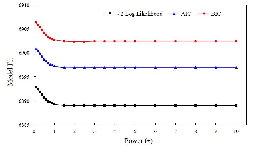
In the case of the model fit comparison by the power (x) of distance (Figure 1), x was changed from 0.1 to 10. The model fit statistics, such as -2 log likelihood, AIC, and BIC, indicate that the model fits become better by increasing the power of distance. However, the model fit results were converged, and their difference was gradually reduced after the square of distance (x=2). Also, the location variable was a significant predictor of average attendance from the original value of distance (x=1.0; α₁=.0232, t=2.03, p<.05) to the 10^th power (x=10; α₁=.0309, t=2.08, p<.05). Based on these results of the model fit comparisons and simplification of the equation, the optimal power (x) of distance was determined as two (x=2) for the analysis of the distance effect between the stadium and the city on MLB attendance, and the location model of an MLB stadium was determined as follows:

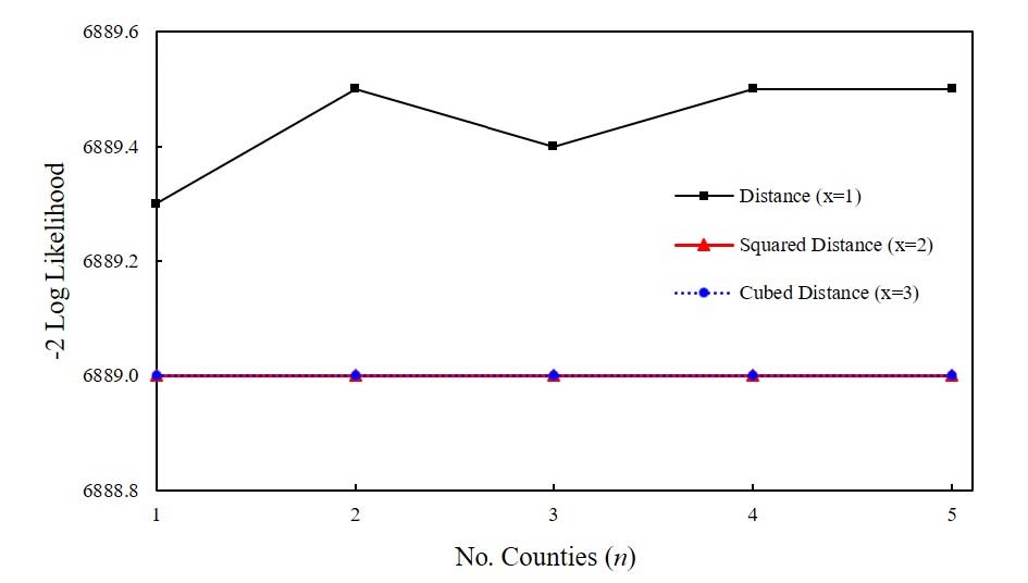
Based on the results of the model above, the other model fit comparison was conducted for finding the optimal number (n) of counties to influence MLB attendance. Figure 2 shows that the model fits (i.e., -2 Log Likelihood when x=1,2,and3) are stable when the number of counties is increased. Therefore, the optimal number of counties for the location variable was one (x=2, n=1; β₁=.0247, t=2.11, p<.05). This result showed the MLB attendance was principally influenced by the demographic and geographic factors of the county that stadium is located.

From the decision of the optimal number of counties, the demand-weighted location model of a stadium was determined as follows:

Based on the results of the optional location model above, 14.8% of the variance by differences between teams was reduced by location variables (τ_o²=42,122,476) while the variance by seasonal differences wasn’t changed (σ²=17,445,840) because most MLB teams had not changed the location of their home stadium during 2006-17 seasons. Even though six MLB teams (i.e., Atlanta Braves, Miami Marlins, Minnesota Twins, New York Yankees, New York Mets, and Washington Nationals) relocated to another stadium during this period, only the Braves and the Marlins moved to a new stadium in the different county.

In addition to this location variable, other attendance determinants in four categories were adopted in this study, and the descriptive statistics of these variables during the 2006 to 2017 MLB regular seasons are shown in Table 3.

Before the analysis of the relationship between MLB attendance and attendance determinants, including the location variable, the data centering by grand means was applied. Table 4 indicates the results of the null model, location model, full model, and final model.

From the likelihood ratio tests for fixed effects of the full models, the final models were suggested. Among the 14 independent variables, 8 variables (i.e., Location, FinalRank, Playoff, TeamAge, Champs, STD_Age, ProTeams, and Season²) were excluded at the full model of MLB attendance model. Per these results, the final model of MLB attendance model was suggested as follows:

In addition, Table 4 shows that the six independent variables (i.e., home team’s final winning percentage, average payroll, and number of star players, stadium capacity, average ticket price, and number of seasons played) significantly influenced each team’s seasonal average attendance from the 2006 to 2017 MLB regular seasons.

Especially, the season final winning percentage (γ₁₀ =20210, t=7.07, p<.001), payroll (γ₂₀=.0023, t=11.87, p<.001), and number of star player (γ₃₀=284.4, t=2.05, p<.05) of teams positively affected the seasonal MLB attendance. Furthermore, the effects of stadium capacity (γ₄₀=0.55, t=7.57, p<.001) and ticket price (γ₅₀=79.68, t=2.02, p<.05) on attendance were significant. However, the recent season’s attendance had been gradually decreased by years (γ₆₀=-570.8, t=-9.89, p<.001).

To check the global fit of the final model, R² measures were adopted in this study. Based on the variance between seasons, and between teams, R₁² and R₂² were measured, and R₁² indicates that the proportional reduction of prediction error by the final model six independent variables is 68.3%. Also, R₂² shows that the prediction error of MLB attendance would be reduced to 72.6% if season i is fixed and team j is randomly chosen, while R₁² and R₂² of the location model are 10.9% and 14.4%.

The purpose of this study was to investigate the effect of stadium location on attendance for the optimal MLB stadium location modeling. For this analysis, two-​level hierarchical linear modeling was adopted because the structure of data had the feature of the nested data (i.e., 12 seasons and 29 MLB teams). Through the analysis of the variance structure by the level of difference, this nested data structure was confirmed. In addition to the two-level modelling approach, this study is the first attempt to investigate the optimal location of stadium related to attendance, and the location is expressed by population, income, and distance between stadium and population center. Even though several studies have adopted the distance from the home team stadium to the nearest other stadium (Winfree et al., 2004), and between the home team and the visiting team (DeSchriver & Jensen, 2002; Lemke et al., 2010), these variables have been investigated as an indicator of other options that might be available for viewing other games and rivalry games rather than as factors of stadium location, which was the focus of the current study. Nelson (2002) analyzed the influence of stadium location in downtown, edge, and suburban areas, but that study was focused on economic gains or losses rather than on the attendance factor examined in the present study.

From the results of location modeling in this study, the seasonal average of MLB attendance was found to be in inverse proportion to the squared distance. Such a finding reveals that distance should be considered as a significant variable, and a short distance between stadium and population center leads to increased attendance. This also suggests the importance of investigating the county in which a sporting facility is located. Although the outcome of the optimal locating modeling is the first attempt of stadium location modeling, it is an approximation and has limitations. Because the units of population, income, and population center in the present study are related to the county instead of the city or the smallest administrative district, and the size of the county varies by state, the results of the data of these slightly larger units and different sizes are limited in terms of accounting for the attendance at all MLB stadiums. In addition, although this study did not include the results of the analysis that included income level and population of city instead of the location factor, the results revealed that income was a significant predictor of MLB attendance, whereas population was not. Because of the location factor, which was a combination of significant (i.e., income) and insignificant (i.e., population) variables, it could be regarded as an insignificant predictor of attendance in the final model.

Further, the current study confirmed the general fact that when teams are looking to possibly move into another stadium, deciding on the new stadium location teams should take into account the population and income of the area. This finding indicates that further study is necessary because of the limitations of the location factors mentioned above. For example, studies using uniform data with no regional differences in units smaller than the county are expected to be a more effective and accurate analysis of the effects of location factors. Also, it is necessary to investigate the location of individual stadiums to reflect local characteristics such as spectator demographics, traffic conditions, and parking conditions in each area. Furthermore, because the effects of the location of stadiums could vary depending on sports such as daily based (e.g., baseball, basketball), weekly based (e.g., soccer, football), and other periodical sporting events (e.g., motorsport), research on various sports is needed. Thus, future stadium location modeling investigations looking into other sports can build up on this study by analyzing other sports and sport industry situations.

In addition to the location factor, several other attendance determinants of the four major categories have also influenced attendance during MLB regular seasons. In the attractiveness factors, the home team’s quality (i.e., winning percentage) and popularity (i.e., average payroll, and star players) influenced attendance from the 2006 to 2017 MLB regular seasons. Several studies have also emphasized the significant influence of the home team’s quality and popularity on attendance (e.g., Carmichael et al., 1999; Hansen & Gauthier, 1989). The results of the current study confirm the importance of the home team’s quality and popularity as they both relate to relates to increased attendance. However, some variables related to the home team’s attractiveness were found to be insignificant predictors if those variables are minutely examined for a specific season. For instance, the home team’s playoff appearance was the only significant predictor of attendance in the 2014 MLB season (Lim & Pedersen, 2018), and other home team attractiveness factors were not. Even though these variables were found to not have statistically influenced attendance on certain occasions, the findings of this study reveal that the variables related to the quality and popularity of the home team are significant predictors of the MLB attendance.

In the residual preference factors, the stadium capacity is a significant predictor of MLB attendance. Stadium capacity is regarded as an indicator of viewing quality (e.g., crowdedness). While some studies are unable to demonstrate the significant influence of stadium capacity on attendance with regard to the MLB (e.g., McDonald & Rascher, 2000), Ferreira and Bravo (2007) found that stadium capacity positively influenced Chilean soccer league attendance. With regard to stadium age, however, the current study was unable to explain the results of previous studies (e.g., Coates & Humphreys, 2007) that noted that the novelty effect of stadium encourages sports fans to attend sporting events. If the variable of stadium age in this study were reflected in the historical worth of stadiums such as Fenway Park (Boston Red Sox) and Wrigley Field (Chicago Cubs), the results would confirm the importance of novelty effect and historical meaning (Coates & Humphreys, 2007).

The elasticity of ticket price of sporting events has been a controversial issue for some time. The negative elasticity of ticket price in various sports leagues has been shown in several studies (e.g., Coates & Humphreys, 2007; Simmons, 1996), and these results accord closely with the microeconomic price theory that is at the heart of the relationship between demand and supply. However, Baimbridge, Cameron, and Dawson (1995, 1996) noted different results with regard to English rugby and soccer. The current study also revealed the positive elasticity of ticket price in MLB attendance. To understand this positive elasticity, it is necessary to compare the attendance demands of 30 MLB teams because it is possible that the popular teams, such as the Red Sox, Yankees, and Cubs, have increased their ticket prices more so than other teams because their fans’ high attendance demands warrant the price increase. The team popularity ranking (The Harris Polls, 2015) and the seasonal average attendance data from the 2006 to the 2015 MLB seasons suggest that the correlation of these two variables is .574. This correlation value would be sufficient to support the notion that high popularity leads to increased attendance, and this would in turn encourage popular teams to raise their ticket prices. The present study is limited with regard to its analysis of the relationship that might exist among demand, attendance, and ticket price because this is not the main purpose of the current study. In order to examine this relationship, additional data and a different research methodology would be necessary.

The season was adopted as variables of longitudinal terms and attendance in the years near the end of the study’s timeframe gradually decreased. Because many MLB teams still depend on the revenue brought in through gate receipts, this decrease in attendance could expose MLB teams to financial risk. Therefore, the league as a whole (MLB) and the individual teams within the league should be concerned with this decrease in attendance, and a study whose purpose is to investigate this trend of decreasing attendance should be conducted as soon as possible.

This study adopted the 14 independent variables, including the longitudinal and quadratic variables (i.e., Season, and Season²) and the location variable, formulated by population, median income and distance, for an analysis of MLB attendance. However, some limitations remain. As previously mentioned, the unit of location data should be small and consistent because there was a variation in the size of the counties examined in this study. Furthermore, the location modeling in this study did not reflect the specific accessibility conditions of each team (e.g., public transportations, parking availability and price, traffic and road conditions). Because these conditions vary with cities, investigating the stadium location of each team or city is something that would be of value in future studies. Moreover, the detailed and precise data related to population, income level and population center would contribute to an even more robust description of the relationship between attendance and stadium location.