Empirical Study on Linear, Non-linear, and System Dynamics: Oriented Human Motor Behavior

Feedback Loop

Force control for motion is induced by the CNS and results in movement through various processes. CNS nerves use command signals called control parameters, provided solely by the person who performs a motor behavior and cannot be changed under the influence of external factors or peripheral information. Here, a signal provided independently of its result is called a feedforward or open-loop control. For instance, when a player hits a ball in a ball sport, the brain sends commands to the muscles. Further, the movement thus generated can be executed regardless of whether the player hits the ball or allows a prediction of its result before confirmation.

By contrast, a signal transformed by the controller depending on the self-generated result is called feedback or closed-loop control. An essential element of this type of control is the comparator (or reference) (Adams, 1971), which allows a comparison between the actual and desired effects. For example, when cycling, the cyclists rely on sensory information to obtain information about their speed from the passing wind or external moving environments and adjust their command signals to decide whether to pedal faster or slower or use the brake. This type of control also allows the cyclists to maintain their preferred speed. This achieves the functional purpose of reducing or increasing errors using the ratio of change in an environmental variable (Δ/Δy) through a positive or negative feedback loop.

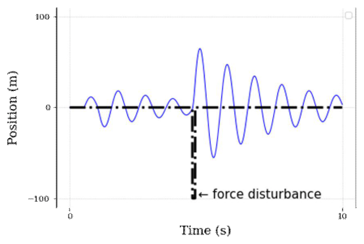
A typical function of a negative loop is to reduce the initial deviation, whereas that of a positive loop is to add a certain proportional number of control parameters to the deviation of the environmental parameter, which leads to the maintenance of a specific value of the output parameter. However, a significant delay can occur in unexpected situations. For example, in the case of perturbations by an external functional signal or feedback loop under a stable state, a complete compensation for the external functional perturbation needs to be achieved through sufficient error correction (Figure 1, left). Furthermore, its failure can cause delays, leading to unexpected results (Figure 1, right). This response delay is a significant drawback of feedback control; it has strong explanatory power for a task requiring a long time or high accuracy but weak explanatory power for an unexpected intervention or fast movement (Schmidt & Lee, 1999).

Figure 1

Representative experimental simulation of the estimated cumulative feedback function. The x-axis denotes the time steps, and the y-axis refers to the control function. The set of left plots denotes a uniform distribution with the function (+1) and its result. By repeating the same property with the perturb function [(+1)*p(−1)], the construct becomes a delayed and non-static result (shown in the plot on the right).

In addition, open- and closed-loop control mechanisms combine contrasting actional characteristics. When applying them to a basketball or soccer game, open-loop control allows a player to snatch the ball by predicting the next move of the opponent. Moreover, closed-loop control executes accurate movements based on the present ball movement, relying on sensory information. These control patterns are attributable to a servomechanism (see Appendix 1’s image on the left side for more detail) consisting of muscle spindles (alphaMNs) and a γ-system (gammaMNs), which is a neurophysiological muscle reflex mechanism that produces spontaneous movements from a control circuit combining different schemas (Matthews, 1972; Merton, 1953). Using an open-loop scheme, the controller sends signals set to static values to the servo loop (tonic stretch reflex or TSR loop), measures the difference between the actual and set values (Δ = X1–X2) with the aid of a feedback mechanism. Through this process, errors are indispensable for the servo function. While an experienced servomotor instantly corrects any deviation, a novice servomotor frequently lags and makes mistakes. This is attributable to the auto-control mechanism of the set value within a specified range. For example, in an isometric contraction, the muscle activity (X) is set to a level enabling continuous maintenance by the comparator, causing a spontaneous increase (X↑) or decrease (X↓) in activity when the difference between the actual and set loads (Δ = X1–X2) exceeds a certain level.

However, muscle activity control in spontaneous contractile movements may not be a hierarchical or independent activity in which a feedback mechanism corrects the deviations in an encoded signal transmitted from the center through an open-loop scheme. While maintaining the position of the elbow through bicep muscle activation to resist an external load, the electromyogram signals of the relevant muscle disappeared for a certain period when the load was abruptly removed (unloading reflex) (Vallbo, 1971). However, the muscle resisting a load through a CNS command should maintain its activation level according to the mechanism based on the above hypothesis. This experimental proof, i.e., extensive stretch reflex (Matthews, 1972), is a limitation of the force control hypothesis (i.e., feedback loop and servo hypothesis) in explaining the motor control performed by the human body. Thus, it has shifted the attention of researchers to a more attractive alternative hypothesis.

Equilibrium Point

A gymnast on a high bar can form a suspended and swaying motor structure using the elastic forces of the muscles interacting with the gravitational force.

Here, m = mass, g = gravity, k = muscle stiffness, p_i = position of mass defined as i in the x_i – y_i relationship, a_ij = value of the mass (i ) added by the intrinsic properties of the muscle (j ), and l_ij = length of the relaxed muscle. When the body hangs on a high bar, the state of the muscles (U ) is formed by the equilibrium configuration between the potential gravitational energy and the potential elastic energy stored in the muscle. This phenomenon (i.e., isometric = total potential energies of the system), which involves a coupling affecting the muscle length and force until reaching the equilibrium point (equilibrium configuration), is appropriate for CNS commands (elastic potential of the spring), and external loads (gravitational potential of the mass) are reached (Asatryan & Feldman, 1965; Feldman, 1966; Latash, 1993) (see Appendix 1’s image on the right side).

As illustrated through a feedback loop, muscle reflexes are utilized when muscles are activated to characterize the parameters of reflexes that change along with the CNS commands. Because this process is backed by the unrestricted control capacity of the reflex circuit, it can overcome the limitations of the feedback loop or servo control hypothesis mentioned above. Furthermore, it can be appropriately applied to all reflex effects of a spontaneous muscle activation. Moreover, the coupling of internal and external factors reflects the nonlinear form (invariant characteristic) of the equilibrium point hypothesis for muscle control mechanisms (Feldman, 1965, 1986; Feldman & Levin, 1995; Latash, 1993).

According to a detailed report related to a hypothesis quantifying the changing relationships between the elementary (force) and performance variables in a similar coupling context (Latash, 2000), motor control occurs synergistically among various elementary variables in achieving a goal.

Elementary variables involved in achieving the goal of a given movement can be good or bad. In Equation (2), to index their relative amounts, V_UCM, i.e., the variance of the uncontrolled manifold (VUCM), is a variance that has no effect on the performance variables and corresponds to a coupling between elementary variables. In addition, V_ORT, the variance in the space orthogonal to the UCM space (VORT) induces its effect on the performance variables for problem posing and corresponds to performance errors between elementary variables. Moreover, V_TOT denotes the total variance (V_UCM+V_ORT), and n is the degree of freedom of the entire space (n=df_UCM+df_ORT). This hypothesis includes the possibility that the index reflecting the goal to be achieved (ΔV) is determined by V_UCM (good variance), which does not affect the performance variables (Scholz & Schöner, 1999). Therefore, control depends on the extent of synergy among the elementary variables to achieve the intended motor behavior.

The above hypothesis, which indexes goal-directed synergy considering neurophysiological mechanisms, demonstrates that the pattern of force required for movement cannot be quantified as a single structural output of the CNS. In addition, it suggests that the main issue should be expanded from an analysis of only elementary units to determine what controls motor behavior. This may be understood as suggesting that given that the force pattern (control) is combined with other fluid variables, the threshold of the invariant characteristics is nonlinear (Schöner, 2002). Moreover, there is a functional and anatomical collaboration between elementary variables, including balanced signal combinations of all spinal nerve forms (Turvey & Carello, 1996).

Point Attractor

Research on nonlinear dynamics began in the 1960s using nonlinear equations (Haken, 1987). Returning to a gymnast swinging on a high bar, suppose the gymnast’s body sways significantly once and then less the next moment. The primary conditions, such as the stiffness of the arm muscles with the gymnasts’ hands hanging on the bar (with stiffness k), gymnast’s mass (m), and friction between the hands and bar (b), are generally equal. The gymnast’s cyclic sway varies depending on the extent to which the gymnast pulls and releases their body when hanging on the bar (position x, velocity x′, and acceleration x″). The harder the pull is, the longer the oscillation, whereas the weaker the pull is, the shorter the oscillation. In both cases, the initial pull eventually ceases. Despite the different durations and shapes, the phenomenon that applies to both cases is a reduction of the energy generated by the pull when swaying toward a nonlinear damping of the oscillation. In both cases, the initial pull eventually ceases. Despite the different durations and shapes, the phenomenon that applies to both cases is a reduction of the energy generated by the pull when swaying toward a nonlinear damping of the oscillation with a gradually diminishing amplitude.

This system phenomenon of converging to a static equilibrium point is termed a “point attractor.” (Kugler et al., 1980).

A movement has multiple spatiotemporal paths and trajectories, depending on its initial state or disturbance (Figure 2). However, the system soon converges to a specific preferred state (damping or pumping) according to the general tendency to maintain a state with low variability and high stability for energy efficiency (Saltzman, 1985). This general characteristic is termed nonlinear attractor dynamics.

Figure 2

Simulation of different attractors. Damped (or pumped) decay lines indicate an embedded invariant property in the relationship between system attractor and damping (or pumping) potential. Dotted line = reference point.

For example, when we lift our fingers or limbs and move them in-phase (Figure 3, left) or anti-phase (Figure 3, center), we can comfortably maintain the phase. If we then move the oscillators (fingers or limbs) at a different pace (Figure 3, right, where one limb has an oscillation frequency of 1 Hz, and the other has a frequency of 0.25 Hz), the phase changes owing to the eigenvalue of each oscillator, and this out-of-phase mode is less comfortable than the in-phase or anti-phase mode. This is due to the increased coordination variability, with the energy consumption increasing to maintain the eigenvalue of each oscillator. Varying the phase coordination requirements signifies that our movement system converges to the preferred state, that is, in in-phase or anti-phase mode, as in the oscillation motion of our example. This is termed a point attractor (Pikovsky et al., 2001), which is a purely stable pattern that appears during the locomotion of the limbs, head, and body.

Figure 3

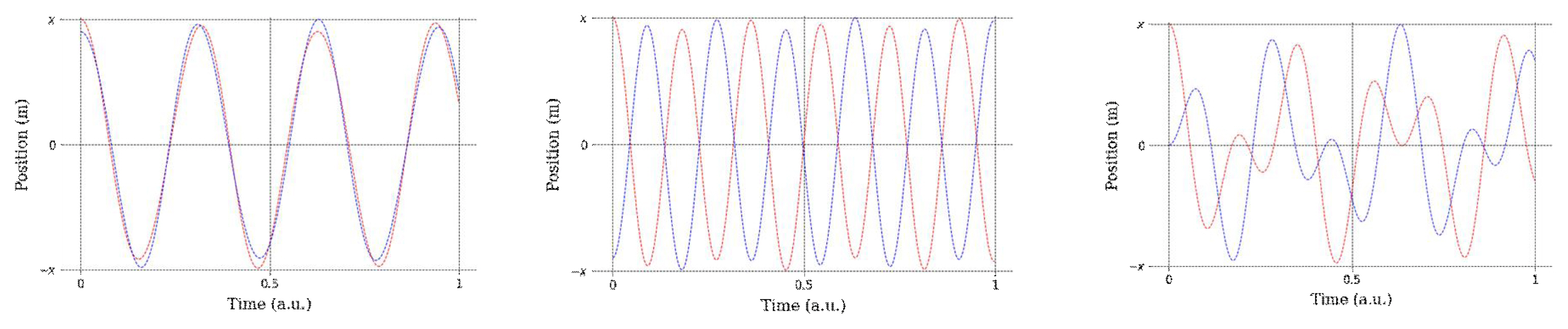
Experimental representation of synchronous diagrams from two different oscillators (red = oscillator 1, blue = oscillator 2): Left = synchronized almost in-phase, with a phase difference; middle = anti-phase condition; right = unmatched initial input between objects (a.u. = arbitrary unit). Note that all the structures were created through a circular function to clearly show their differences.

Table 1

Data collection for experiment

Elementary Coordination

This property of invariant dynamics is the limb oscillation coordination characteristic of human motor behavior and constitutes the basis for explaining the regular locomotion of the limbs (Kay et al., 1987). The phase of an oscillator can be quantified by adding the time-dependent phase angle [ω₁(t)] at the point where the oscillator motion begins [θ₁(0); see Appendix 2 for more details of the schematic depiction), where r is a constant. When similarly estimating the phase of the other oscillator (θ₂), [ω₂(t) + θ₂(0)], the relative phase of the limbs is stable when in-phase (θ₂ - θ₁ ≈ 0) or anti-phase (θ₂ - θ₁ ≈ π).

Our limb coordination system prefers in-phase (φ ≈ 0) mode (Figure 4, reconfirmed by the Haken-Kelso-Bunz (HKB) model) (Haken et al., 1985). Moreover, when the energy demand [movement speed = control parameter (V)] required for coordination stability, such as an increased speed in basic symmetrical motion, increases, the anti-phases of the upper and lower limbs show a relatively unstable pattern. This is because the energy demand increases up to a certain point where a sudden shift to the in-phase mode occurs. By contrast, this phase transition, according to the energy demand, does not always occur under in-phase mode. There is also no phase transition under the same phase because of the energy demand (Kelso, 1984).

Figure 4

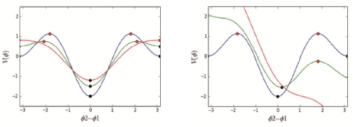
Schematic of the experimental conditions and results of different phases: Left = general experimental setting with apparatus; middle = plot; right = the observed relative phase or phase relation between two oscillators at φ≈0 deg (in-phase) or φ≈ ± 3.14 deg (anti-phase = π). The movement speed denotes the control parameter, and the arrow indicates the attractor. In the plot on the right, V is the intrinsic dynamics of the potential function, and the black balls symbolize stable states (attractors) and red balls correspond to unstable states (repellers), φ2–φ1 ≈ 0 denotes a condition of a nearly synchronized in-phase, and φ2–φ1 ≈ π indicates a condition of an anti-phase.

Here, φ is the phase angle of each activated limb oscillator, - φδω is the difference in the eigenvalue of each oscillator, and α and b are the coefficients of the two limbs, indicating the coupling strength. Equation (6) describes how the relative phase (φ), which represents the difference in the phase angle between two limbs, is determined based on the relative coupling strength according to the ratio between the two coefficients (α/b) (Kugler & Turvey, 1987). It experimentally reflects the nonlinear preferred stability that appears in our coordination process, that is, the attractor of the potential function (see Appendix 3 for more details) (Haken et al., 1985).

In addition, the symmetry of movements derived from the empirically tested nonlinear “point attractor” is spatiotemporally broken depending on the structure and function of the body (Amazeen et al., 1998). This is because routine coordination (e.g., grasping, twisting, and manipulating) involves our limbs and occurs in various ways due to the voluntary (or imposed implementation of) numerous interactions (Collins & Stewart, 1993). Therefore, to explain the coordination pattern and transition characteristics, we extended the basic theoretical model, which can be implemented by breaking the symmetry through frequency competition (Δω=ω_L-ω_R) (Amazeen et al., 1998) in the interlimb coordination model (Haken et al., 1985).

It was also implemented without symmetry, breaking through the asymmetric coupling of the interlimb eigenvalues (=Δω) or coupling intensity (coefficient of b/a) by expanding the coordination asymmetry (preference (dominant arm), attention, and oscillator axis of rotation) (Treffner & Turvey, 1996). For instance, based on the interlimb coordination defined by Equation (6), condition-dependent differences in the coupling intensity of the additional variables under examination were quantified through symmetry breaking (|c and d|>0, |c and d| ≈ 0) to examine their relative differences in phase.

In the expansion (Equation (7)), ϕ̇ = change in the relative phase, Δω= the extent of disequilibrium through the eigenvalue of each oscillator, [a cos(ϕ)+ b cos (2ϕ)] is the extent of equilibrium defined at an oscillation value of 0 or π (= inter-oscillator coupling intensity, and ρ = Gaussian white noise, i.e., asymmetric coupling attractor (= [α sin(φ) + 2b sin(2φ)]) intentionally added to the basic interlimb coordination structure (Amazeen et al., 1997; Park et al., 2001). Such applications have enabled us to examine from various angles how essential coordination dynamics are microscopically manifested through asymmetric potentials (see Appendix 4 for more details) (Park, 2020). We can recognize the dynamic structure of a neurological or behavioral variable as a representative state, as expressed by the mean [φ_ave-φ₀ (rad)] and standard deviation [SDφ(rad)] of the relative phase and the coefficient of variation (CV) [SDφ(rad)/φ_ave-φ₀(rad)].

However, this approach cannot elucidate whether the outputs of a movement or motor behavior of individual elements continuously change within a time series, not to mention the situation itself (Horn & Newton, 2019). This has contributed significantly to our understanding of the nonlinear dynamics of coordination patterns and the structural stability of various movements. At the same time, limitations are inevitable under the methodological aspect of experimental research, such as individual differences, sampling, and time series, in objectively explaining the principles and changing modes of motor behavior (Narizuka & Yamazaki, 2018).

Network-agent-based Evolution

As previously described, system dynamics can show how parts or components jointly shape a structure and adapt to environmental changes. A greater emphasis is placed on the emergence of stationarity than on the accuracy or variability of force control, stability, and coordination uncertainty. Its crucial variables are the actions of other individuals and the environment (i.e., neighbors) interacting with individuals (e.g., molecules, cells, or athletes). With the changes in its state at each given point in time (ȳ_i) being monitored within the time series (g_i(t)) and its components (x) reflecting autonomous agents (b_i(x)) acting in a bottom-up manner, we assign practical meaning to behavior and state (f (χ̄)) (Poggio & Bizzi, 2004; Reynolds, 1987).

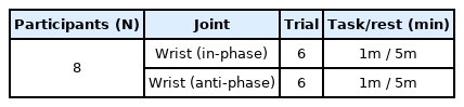
Because it can also include mechanisms exploring and imitating the strategies of other constituent elements (i.e., training habits and a tendency to seek healthcare), it enables more realistic estimates of the change and adaptation process based on interactions (Oliva, 2016). Specifically, many individuals and various components, their organizational form (structure: see Table 2 and Figure 5), and basic properties with constituent elements such as a propagation of positive (payoff) and negative (failure) variables allow more detailed (i.e., simulation) observations of processes such as changes in motor behavior (Pastor-Satorras et al., 2015).

Table 2

Athletes Network structure (Small-world property)

Figure 5

Athlete network topologies from professional athletes in South Korea. The left and right plots depict random and regular structures, respectively. The middle plot depicts the network structure of male baseball players (n = 40, the actual level of support among team members = 5.5, and the actual level of support outside of team members = 0.18). These topologies were created using the parameters n = individual, p = regular connections within the team, and β = random connections outside the team. The questionnaire had a simple question regarding who would support the player (or contact) when having important matters to discuss (e.g., injury, advice, mistake, necessary decision-making, or poor behavior).

The significance of this system dynamics approach (i.e., network and agent-based simulation) is emphasized in sports-related research (Clemente et al., 2016). Furthermore, its effectiveness has been demonstrated through myoneural activity (Ryan et al., 2018), sports performance transfer (Bock et al., 2012), and outcome prediction (Bunker & Thabtah, 2019; Oldham & Crooks, 2019). This implies that studies have examined complicated intra- and inter-system interactions between individuals rather than observing the relationship between a force and interlimb coordination (Glazier & Davids, 2010). We previously verified empirically that our movements or motor behaviors are formed by the relative hierarchy of the CNS or its components and arise from the relationships between organizational members, whereby the role of influential individuals can serve as the strategy of that organization (system) (Passos et al., 2017).

According to Newell (1986), who investigated the principles of human motor behavior in the same context, the action of dynamic systems, such as human movement and motor behavior, emanates from interdependent system constraints between individuals, tasks, and the environment. Performer limitations such as motivation, skill level, or physical and psychological characteristics; task limitations such as rules, methods, and performance goals; and environmental constraints such as stadium conditions, jet lag, and sociocultural differences are inevitable constraints constantly encountered by performers. Furthermore, information constraints, such as the awareness of a performer regarding an individually available situation under a specific spatiotemporal setting, also affect decision-making at any instant. When encountering these constraints, we must appropriately interact with the constraining factors under other states for a successful task execution (Araújo & Davids, 2016). Therefore, the systematic handling of these relationships provides a realistic and accurate understanding of the phenomenon of motor behavior. Specifically, it captures the complicated interactions between components and the centrality of patterns and movements, and then analyzes intra-system interactions (Korte & Lames, 2018; Sampaio & Leite, 2013).

The following findings are noteworthy: (i) Functional variables of numerous nerves and muscles interconnected to produce movements (Grillner, 1975) are characterized by systematically different network properties (i.e., visual and motor systems) (Georgopoulos et al., 1982).

The visual system (Equation (12.1)) is a set of regulated unity activities [A = matrix(eigenvalue), k_i (χ̄ ) = vector(eigenvector)] and mostly derives a single output signal (f̄ (x )) (Figure 6, plot on the left side). By contrast, the motor system (Equation (12.2)) regulates the unit activity of the individual components, and various types of output signals appear as the output vector field (f̄ (χ̄ )) or activations in parallel (f̄ (χ̄ _j )) (Figure 6, plot of the middle side). However, regardless of the origin (i.e., top-down or bottom-up) and destination (i.e., ā→b̄→c̄, b̄→c̄→ā, ..., c̄→ā→b̄) of a signal stimulus and its output mode (single, as the visual system, or multiple and parallel, as the motor system), all possible interactions are formed as networks of the matrix (A ) and vector k_i (χ̄ )) (Wickelgran, 1969) (Figure 6, plot on the left and middle). Even if the action of each component of a different structure is perceived with different intensities (i.e., centrality) depending on the constraints, they are positively or negatively interconnected and affect each other. Thus, a problem in any component results in a structural stability loss in the functionality (Sussillo et al., 2015).

Table 3

Descriptive network property and its adjacent matrix for football data

Figure 6

Generalization architectures of motor systems. In the case of vision (left), a single output signal is a combination of tuned unit activities (with weighted edges of a node). In the case of motor control (middle), each component of the output field is a combination of tuned unit activities (with weighted edges of a node). The right side shows its adjacent matrix corresponding to the network connection scheme. The plot of the right set shows a created team sport passing the network property of football data (average value on successful passes). The tracking of the passing distribution at the FIFA World Cup 2014 tournament was provided in the official FIFA match reports on their website (WorldCup/archive). The plot of the football shows that a defensive midfielder is significantly more central (P < .05) than other positions (see Table 3 for more details). Note a set of nodes connected by ties that link them (x_ij defines a binary tie between nodes).

(ii) These network properties estimate the central tactical position during the game, based on the frequency and success rate of passes made in team sports such as soccer, basketball, and handball by expanding the scope of the application (Korte & Lames, 2018) (Figure 6, plot on the right).

(iii) Athletes mimic, unconsciously and automatically, the momentary emotional expressions of their teammates (Barsade, 2002). Furthermore, the positive or negative mood of a person (athlete or coach) rapidly spreads to other team members, exerting significant effects on their collaboration, conflicts, and task performance (Barsade et al., 2018).

(iv) In addition to changes in the form and injuries, small and large incidents, such as significant changes in individual performance (sports streaks (Bar-Eli et al., 2006)) were observed to considerably impact the functionality of the system (Thacker et al., 2003). We must estimate such system dynamics in a myoneural network with a high interconnection of the components (Pacheco et al., 2006).

Because an individual can be identified by a specific arrangement (n × m) of interdependent relationships within the matrix of the network components to which they belong, more specific and direct content at issue is investigated, such as the connective structure, degree, hierarchy, and centrality. As empirically illustrated in Figure 6, a structure similar to a sports team that forms a low variance at an extremely high degree of interconnection has an exponentially faster and higher risk transmission rate (see Appendix 5 for more details) than a general social structure that does have such a formation (Cui et al., 2021). This system dynamics model has also been applied in situation to basic motor behavior (Park, 2020). Furthermore, the phenomenon of an emergent pattern of key debates of individual movements (i.e., velocity and displacement) was also empirically observed (Figure 7, right) by adding mechanical variables (i.e., imitation and exploration) that can be estimated from simple individual movement characteristics (Figure 7, left: movement).

Figure 7

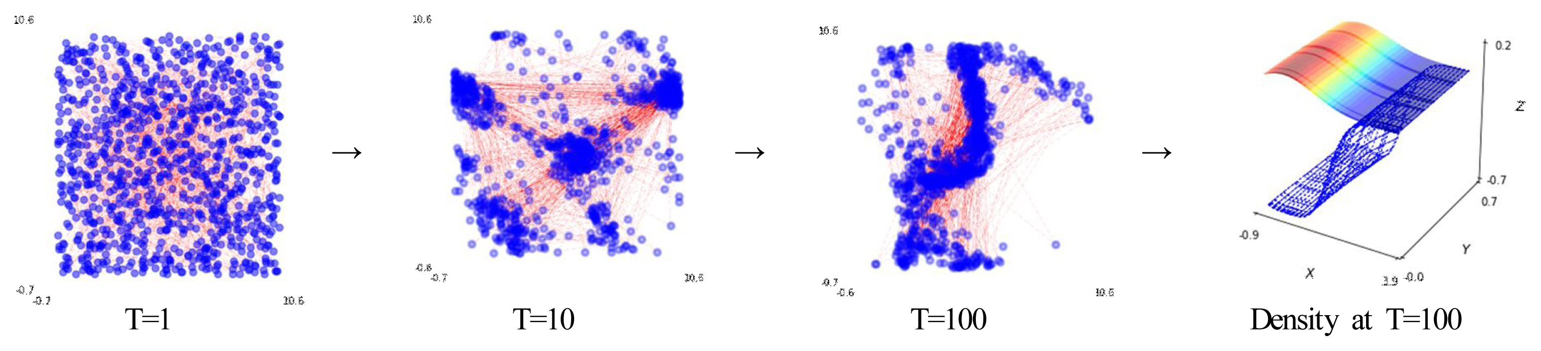
Behavioral dynamics underlying the network structure (see Table 2) and simple movement rule. Based on the simulation, the plot on the left shows that a displacement separates the individuals at the initial time steps (T = 1), and the relative position structure is controlled by the initial setting. Blue dots represent their position in an x, y coordinate plane, and the red lines denote links. The middle plots show the dynamic influence based on the individual characteristics at T = 10 and T = 100 (middle right). The right plot represents its behavioral bias calculated by the density function (T = time steps). It refers to the fact that although the pattern of the individual behavior depends on a localized view of the initial conditions, a slight change in the individual movement characteristic (velocity) has a remarkably diverging (or converging) displacement.

Complex Behavior

Reverting to the action of forces for more direct relevance to the principles explaining movements and motor behaviors, system dynamics (Haken, 1987) is of particular importance. Inspired by nonlinear dynamics studied during the 1960s, system dynamics characterized the concept of force as an elemental low-energy force field that directly forms a motion and can be applied to all systems as the motion and direct time-dependency change. This is because a slight change in force under the initial state leads to a small change on a short time scale but results in a qualitatively dramatic change on a longer time scale, drawing attention to the change in energy flow in tandem with a change over time rather than the force itself (Kugler et al., 1980). Specifically, the force can be viewed as a dynamic phenomenon inherent in a system governed by a self-recursion rule, rather than simply as a static state, such as the position (x) or velocity (x′ (Rosen, 1987, 1991)).

Movement is not simply a change from one position or velocity to another (x_o, x_{o ′}), but rather a phase change (x_o +x_{o ′} dt, x_{o ′}+Fdt) under a constraint in which individuals, tasks, and environments interact to a limited extent (Bohm, 1969). This represents the view that an individual cannot reach the goal intended by the motor behavior by individually producing all forces required for implementing a task or motion but rather contributes to the flow of the total energy by being involved in the event or direction of concern.

This conceptual or methodological application of system dynamics (i) can estimate the extent to which the phase or relative pattern of a motor behavior within a time series is based on the degree of linear or nonlinear stability, which gradually changes. For example, (ii) based on a linear mean or standard deviation, system uncertainty can be assessed using the probabilistic (p_i ) expected value [log (1/p_i )] of each variable (Shannon, 1948).

This is also (iii) a query into structured nonlinear quantitative (Stergiou & Decker, 2011) information on a time-series analysis, including the complexity, which varies according to the sensitivity of the initial conditions of the analyzed object (variable r).

Figure 7 shows the dynamic character of the system (vector operation), which the distance of the basic system phase defined as a given initial property differs in a time series. It denotes the time-dependent attractors’ changes to the parameter of interest and the topographic branching that appears as it passes through a specific time point in the phase space, allowing us to discern the qualitatively different behavioral contributions included in various constraints or motor parameters. The emergent phenomenon that shows the distance in the time-series-defined phase space and the stability (i.e., coordination or cooperation) of the object of observation begins to be driven from the initial state (Figure 8).

Figure 8

Schematic of the individual (vector = v⃗_i, averaged = v⃗_avg ) operation in R².

Notably, this fundamental process indicates that the second quantity of v⃗ contains the trait of the individual (agent-self interactions, where agents can interact with themselves), based on whether the following condition holds:

where the function assumes that the attribute of the component is conditional upon the value yield in the other direction (−) if the length of the magnitude ||v_i|| is greater than the other length (||v_avg||). This trait was implemented according to the following quantities:

where v⃗_i is the velocity of the individual, represented by the length of the individual’s magnitude (||v_i|| ) with the direction of the individual (d⃗_i ). In addition, v⃗_avg is the average velocity, which includes the navigation of the entire population of N individuals. The results of v⃗_i and v⃗_avg produce a new quantity v⃗_inew, which is written simply as (v⃗→v⃗_inew = v⃗_i+v⃗_avg ). This application expands a relatively simple nonlinear equation to gauge the system complexity (Wolf et al., 1985). In addition, we can more elaborately determine the collective dynamic relationships of a group of periodically operated systems.